mlim : Single and Multiple Imputation for R and Stata with Automated Machine Learning

mlim is the first missing data imputation software to implement automated machine learning for performing multiple imputation or single imputation of missing data. The software, which is currently implemented as an R package, brings the state-of-the-arts of machine learning to provide a versatile missing data solution for various data types (continuous, binary, multinomial, and ordinal). In a nutshell, mlim is expected to outperform any other available missing data imputation software on many grounds. For example, mlim is expected to deliver:

1. Lower imputation error compared to other missing data imputation software.
2. Higher imputation fairness, when the data suffers from severe class imbalance, unnormal destribution, or the variables (features) have interactions with one another.
3. Faster imputation of big datasets because mlim excells in making an efficient use of available CPU cores and the runtime scales fairly well as the size of data becomes huge.

Fine-tuning missing data imputation

Simply put, for each variable in the dataset, mlim automatically fine-tunes a fast machine learning model, which results in significantly lower imputation error compared to classical statistical models or even untuned machine learning imputation software that use Random Forest or unsuperwised learning algorithms. Moreover, mlim is intended to give social scientists a powerful solution to their missing data problem, a tool that can automatically adopts to different variable types, that can appear at different rates, with unknown destributions and have high correlations or interactions with one another. But it is not just about higher accuracy! mlim also delivers fairer imputation, particularly for categorical and ordinal variables because it automatically balances the levels of the avriable, minimizing the bias resulting from class imbalance, which can often be seen in social science data and has been commonly ignored by missing data imputation software.

mlim outperforms other R packages for all variable types, continuous, binary (factor), multinomial (factor), and ordinal (ordered factor). The reason for this improved performance is that mlim:

• Automatically fine-tunes the parameters of the Machile Learning models
• Delivers a very high prediction accuracy
• Does not make any assumption about the destribution of the data
• Takes the interactions between the variables into account
• Can to some extend take the hierarchical structure of the data into account
  • Imputes missing data in nested observations with higher accuracy compared to the HLM imputation methods
• Does not force a particular linear model
• Uses a blend of different machine learning models

Procedure

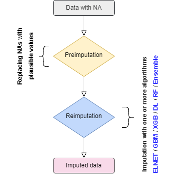
When a dataframe with NAs is given to mlim, the NAs are replaced with plausible values (e.g. Mean and Mode) to prepare the dataset for the imputation, as shown in the flowchart below:

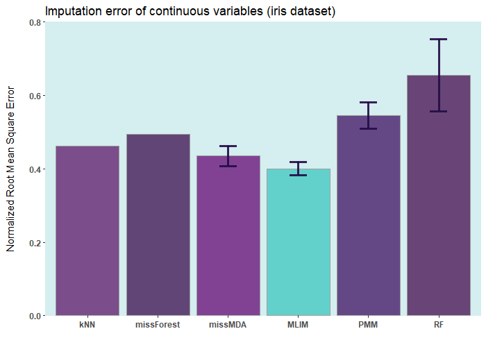
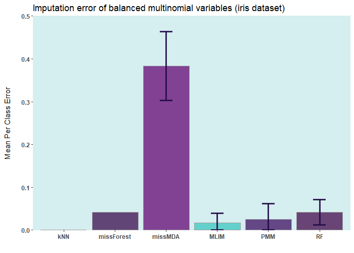
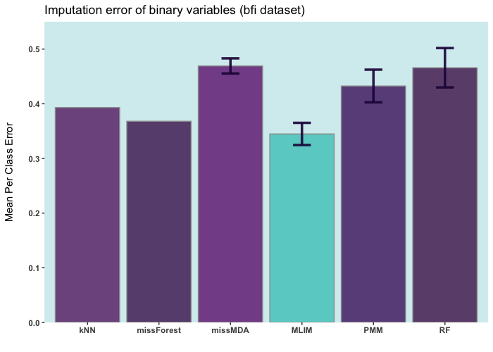
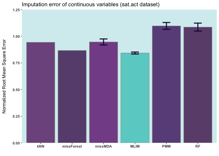
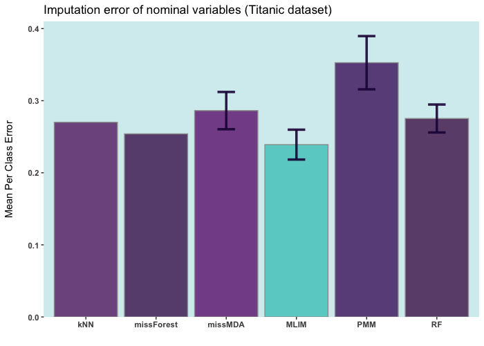
Fast imputation with ELNET

Below are some comparisons between different R packages for carrying out multiple imputations (bars with error) and single imputation. In these analyses, I only used the ELNET algorithm, which fine-tunes much faster than other algorithms (GBM, XGBoost, and DL). As it evident, ELNET already outperforms all other single and multiple imputation procedures available in R language.

R Installation

To install the latest version from GitHub:

library(devtools)
install_github("haghish/mlim")

Depending on the learners you wish to use for imputation, there will be other dependencies. For installing all learners supported by mlim, you will need the following R dependencies:

# Required packages
install.packages(c("partykit", "sandwich", "coin", "gbm", "lightgbm", "kernlab", "kknn", "readstata13", "remotes"))

# Optional packages fot catBoost imputation (for Mac)
remotes::install_url("https://github.com/catboost/catboost/releases/download/v1.2.10/catboost-R-darwin-universal2-1.2.10.tgz",
  INSTALL_opts = c("--no-multiarch", "--no-test-load", "--no-staged-install"))

# Optional packages fot catBoost imputation (for Windows)
remotes::install_url(
  "https://github.com/catboost/catboost/releases/download/v1.2.10/catboost-R-windows-x86_64-1.2.10.tgz", 
  INSTALL_opts = c("--no-multiarch", "--no-test-load"))

# Optional package for catboost imputation (for Linux)
remotes::install_url("https://github.com",
                     INSTALL_opts = c("--no-multiarch", "--no-test-load", "--no-staged-install"))

# Additional learners (RECOMMENDED!)
install.packages("mlr3extralearners", repos = c(mlrorg = "https://mlr-org.r-universe.dev"))

Stata Installation

mlim is also available in Stata. The github package is the only recommended way for installing mlim. Once github is installed, you can install the package with the following command:

github install haghish/mlim

Supported algorithms

mlim supports several algorithms:

• ELNET (Elastic Net)
• RF (Random Forest and Extremely Randomized Trees)
• GBM (Gradient Boosting Machine)
• XGB (Extreme Gradient Boosting, available in Mac OS and Linux)
• DL (Deep Learning)
• Ensemble (Stacked Ensemble)

ELNET is the default imputation algorithm. Among all of the above, ELNET is the simplest model, fastest to fine-tune, requires the least amount of RAM and CPU, and yet, it is the most stable one, which also makes it one of the most generalizable algorithms. By default, mlim uses only ELNET, however, you can add another algorithm to activate the post-imputation procedure.

GBM vs ELNET

But which one should you choose, assuming computation resources are not in question? Well, GBM is very liokely to outperform ELNET, if you specify a large enough max_models argument to well-tune the algorithm for imputing each feature. That basically means generating more than 100 models, at least. But you will enjoy a slight – yet probably statistically significant – improvement in the imputation accuracy. The option is there, for those who can use it, and to my knowledge, fine-tuning GBM with large enough number of models will be the most accurate imputation algorithm compared to any other procedure I know. But ELNET comes second and compared to its speed advantage, it is indeed charming!

Both of these algorithms offer one advantage over all the other machine learning missing data imputation methods such as kNN, K-Means, PCA, Random Forest, etc… Simply put, you do not need to specify any parameter yourself, everything is automatic and mlim searches for the optimal parameters for imputing each variable within each iteration. For all the aformentioned packages, some parameters need to be specified, which influence the imputation accuracy. Number of k for kNN, number of components for PCA, number of trees (and other parameters) for Random Forest, etc… This is why elnet outperform the other packages. You get a software that optimizes its models on its own.

Advantages and limitations

mlim fine-tunes models for imputation, a procedure that has never been implemented in other R packages. This procedure often yields much higher accuracy compared to other machine learning imputation methods or missing data imputation procedures because of using more accurate models that are fine-tuned for each feature in the dataset. The cost, however, is computational resources. If you have access to a very powerful machine, with a huge amount of RAM per CPU, then try GBM. If you specify a high enough number of models in each fine-tuning process, you are likely to get a more accurate imputation that ELNET. However, for personal machines and laptops, ELNET is generally recommended (see below). If your machine is not powerful enough, it is likely that the imputation crashes due to memory problems…. So, perhaps begin with ELNET, unless you are working with a powerful server. This is my general advice as long as mlim is in Beta version and under development.

Citation

• Haghish, E. F. (2022). mlim: Multiple Imputation with Automated Machine Learning [Computer software]. https://CRAN.R-project.org/package=mlim.

Example

iris ia a small dataset with 150 rows only. Let’s add 50% of artifitial missing data and compare several state-of-the-art machine learning missing data imputation procedures. ELNET comes up as a winner for a very simple reason! Because it was fine-tuned and all the rest were not. The larger the dataset and the higher the number of features, the difference between ELNET and the others becomes more vivid.

Single imputation

In a single imputation, the NAs are replaced with the most plausible values according the model. You do not get the diversity of the multiple imputation, but you still get an estimated imputation error based on 10-fold (or higher, if specified) cross-validation procedure for each variable (column) in the dataset. As shown below, mlim provides the mlim.error() function to summarize the imputation error for the entire dataset or each variable.

# Comparison of different R packages imputing iris dataset
# ===============================================================================
rm(list = ls())
library(mlim)
library(mice)
library(missForest)
library(VIM)

# Add artifitial missing data
# ===============================================================================
irisNA <- mlim.na(iris, p = 0.5, stratify = TRUE, seed = 2022)

# Single imputation with mlim, giving it 180 seconds to fine-tune each imputation
# ===============================================================================
MLIM <- mlim(irisNA, m=1, seed = 2022, tuning_time = 180) 
print(MLIMerror <- mlim.error(MLIM, irisNA, iris))

# kNN Imputation with VIM
# ===============================================================================
kNN <- kNN(irisNA, imp_var=FALSE)
print(kNNerror <- mlim.error(kNN, irisNA, iris))

# Single imputation with MICE (for the sake of demonstration)
# ===============================================================================
MC <- mice(irisNA, m=1, maxit = 50, method = 'pmm', seed = 500)
print(MCerror <- mlim.error(MC, irisNA, iris))

# Random Forest Imputation with missForest
# ===============================================================================
set.seed(2022)
RF <- missForest(irisNA)
print(RFerror <- mlim.error(RF$ximp, irisNA, iris))

Multiple imputation

mlim supports multiple imputation. All you need to do is to specify an integer higher than 1 for the value of m. For example, set m = 5 in the mlim function to impute 5 datasets. Then, mlim returns a list including 5 datasets. You can convert this list to a mids object using the mlim.mids() function and then follow up the analysis with the mids object the same way it is carried out by the mice R package. Here is an example:

# Comparison of different R packages imputing iris dataset
# ===============================================================================
rm(list = ls())
library(mlim)
library(mice)

# Add artifitial missing data
# ===============================================================================
irisNA <- mlim.na(iris, p = 0.5, stratify = TRUE, seed = 2022)

# multiple imputation with mlim, giving it 180 seconds to fine-tune each imputation
# ===============================================================================
MLIM2 <- mlim(irisNA,  m = 5, seed = 2022, tuning_time = 180) 
print(MLIMerror2 <- mlim.error(MLIM2, irisNA, iris))
mids <- mlim.mids(MLIM2, dfNA)
fit <- with(data=mids, exp=glm(Species ~ Sepal.Length, family = "binomial"))
res <- mice::pool(fit)
summary(res)